By Dick Kazarian, Managing Director, Borrower Analytics Group
Introduction and Summary
Over the past two years, MIAC’s Borrower Analytics Group has completely revamped the CORE™ Family of Residential Behavioral Models. These models cover all three residential sectors: Agency, GNMA, and Non-Agency and include the following components:
- Credit frequency (i.e., “roll rates”)
- Voluntary Prepayments
- Foreclosure/REO Timelines
- Loss Severity (i.e., Loss Given Default)
Together, these model components provide a complete probabilistic description of all possible outcomes for a given loan at every projection month. These models have been implemented into Vision™ and WinOAS™, our two primary asset valuation solutions. In addition, the data normalization and missing value imputation challenges have been addressed with DataRaptor®, our extract, transform and load (i.e., ETL) software solution.
MIAC’s Borrower Analytics Group has extensive prior experience in model development and model validation at leading investment banks and CCAR commercial banks. We adhere to a disciplined and rigorous model development process. These development phases include (1) data preparation and exploratory data analysis, (2) feature/explanatory factor definition, (3) model specification and estimation, (4) parameter review, (5) software implementation, and (6) replication testing. This process is designed to satisfy the regulatory requirements of SR 11-7 as well as conform with industry best practices regarding model risk management.
The purpose of this report is to highlight the six primary features which distinguish these behavioral models. They include:
- An exhaustive set of explanatory variables
- Incorporation of all relevant macro-economic factors
- Detailed loan status tracking throughout the life of the loan
- A highly granular and macro factor-dependent foreclosure/liquidation timeline model
- A state-of-the-art loss severity model that is fully integrated with the frequency model
- Sub-models that capture distinct intra-sector and product-specific behavior
In forthcoming issues of MIAC Perspectives, we will elaborate on each of these features in much greater depth, provide conceptual and empirical support for our approach, and demonstrate the quantitative impact on outcomes for both MSRs and whole loans.
Feature 1: An Exhaustive Set of Explanatory Variables
All of our models were estimated using the best loan-level data available for that particular sector. Our estimation process considered a large set of potential explanatory variables based on data availability, industry and academic research, and prior experience.
The ideal dataset for a particular sector has all available attributes (i.e., fields), a rich cross-section of those attributes (e.g., a broad range of FICOs, DTI, etc.), and a long history through various economic cycles. However, all datasets have limitations. For example, the GNMA loan-level disclosures have a large set of attributes but a very limited history: the observations start in 2012. Importantly, the GNMA data does not include the financial crisis where mark-to-market combined LTVs (hereafter, CLTV-MTM) reached 200% and higher.
We address these limitations by using both primary and secondary (or supplemental) datasets for each model. For example, the GNMA loan-level disclosure data is the primary dataset because this has the largest population of distinct loan attributes. However, this primary dataset is supplemented with the Agency loan-level data – whose history covers the financial crisis. This secondary dataset enables us to inform our estimation of loan behavior in the high CLTV-MTM region.
The above example shows how we enrich the GNMA data to supplement an observation period deficiency. We also use secondary datasets to supplement missing attributes. For example, we use the co-borrower field in the Agency data to inform our estimation of this effect in the non-Agency model.
Figure 1 provides an overview of the variables included in our CORE Family of Residential Behavioral Models. We also indicate whether or not the cross-section of our behavioral model competitors also includes that explanatory variable. As is evident, our models make use of a larger set of factors than typical competitor models. And as we show below, these additional variables make our predictions more precise.
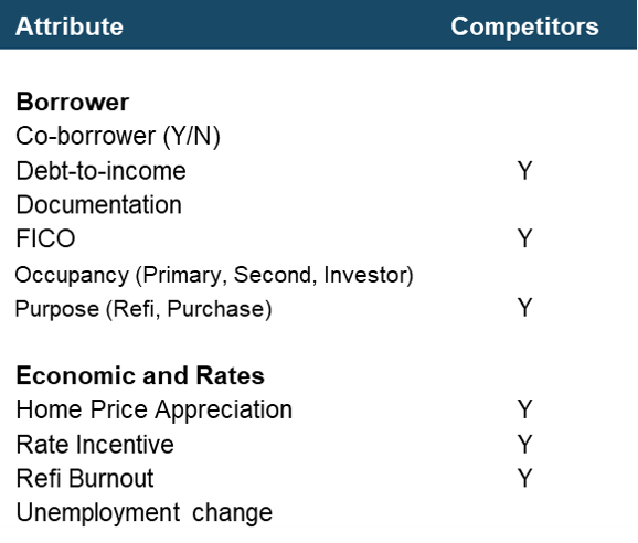
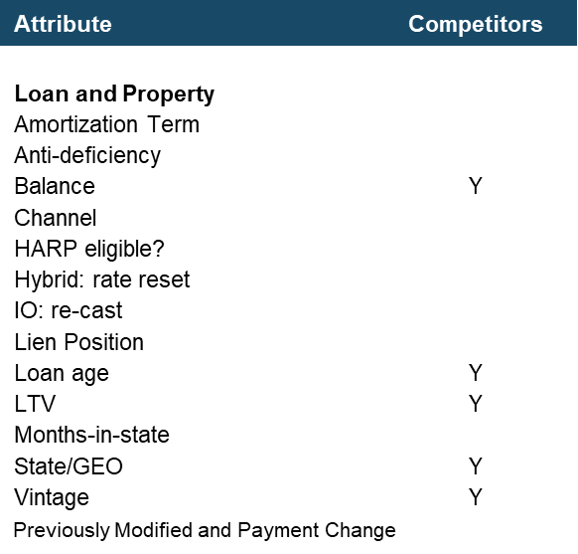
Figure 1: CORE Model Variables Source: MIAC Analytics™
Although a comprehensive set of explanatory variables results in much higher precision, it also requires a much more extensive data management effort to prepare a portfolio for analysis. Otherwise, the advantages of a more sophisticated and accurate model will not be realized. This data preparation effort includes data scrubbing, data normalization, and imputation of missing values. MIAC has 30-plus years of experience handling large sets of mortgage loan-level data. We have the software, reporting, and customer support to handle large, irregular, and otherwise challenging client data. As one important example, we supplement these behavioral models with missing value models which optimally impute the expected value of missing attributes as a function of available attributes. As a result, our analytics can be run on diverse client datasets with widely disparate levels of data availability.
Feature 2: Incorporation of all Relevant Macro-Factors
Mortgage outcomes (i.e., defaults, prepayments, foreclosure timelines, and loss severities) depend upon both attributes observed at (or near) origination (like DTI, FICO, and CLTV) as well as the evolution of macro-economic factors (like mortgage rates, interest rates, home prices, and unemployment).
Similar to many competing models, our CORE models use both primary mortgage rates and home prices to drive mortgage outcomes. Following common industry practice, we use realized historical home price indices (hereafter, HPA) from loan origination through the observation date to update the CLTV-MTM. This updated equity impacts all mortgage outcomes: prepayments, defaults, foreclosure timing, and losses. For example, higher CLTV-MTM generally reduces prepayment rates and increases default rates.
In sharp contrast to many competing models, our CORE models also use the state-level unemployment change (from loan origination through the observation date). Unemployment (hereafter, UER) and home prices (hereafter, HPA) were somewhat correlated during the 2007-2010 housing crisis, leading some researchers to conclude that HPA could reasonably proxy for “economic conditions”. However, there is no question that UER provided significant explanatory power even after controlling for HPA (via CLTV-MTM). The empirical evidence is simply overwhelming, as shown in Figure 2 below.

Figure 2: Impact of UER change on C–> D30 Transition (Agency Fixed Rate) Source: MIAC Analytics™
Figure 2 displays the relationship between monthly Current-to-D30 transition rates (i.e., C->D30) and the change in UER between loan origination and the observation date. For example, a UER change of 2 means that unemployment increased by 2 percentage points (e.g., from 5% to 7%). As is clearly evident, increases in UER result in higher C->D30 transition rates. The results are shown for Agency data, but we find similar results for all Sectors and most transitions. Further, the marginal effect of UER is large and statistically significant even after controlling for HPA, which is handled through our econometric specification.
A few additional points merit consideration. First, Figure 2 also shows that our CORE model for C->D30 fits the data quite well. In other words, there is no systematic pattern between actuals (shown as the dots) and predicted (shown as the fitted line). Second, the current COVID-19 crisis underscores the importance of using both UER and HPA as macro drivers: UER has been very volatile, while HPA (along with other asset prices) has been increasing rapidly.
Third, we have conducted extensive additional econometric testing of numerous other potential macro-economic factors, such as disposable income and population changes. Our research shows that these additional factors do not have any marginal explanatory power. In technical terms, we have found that UER is both necessary and sufficient for explaining loan performance.
Feature 3: Detailed Loan Status Tracking
Our CORE Residential Models provide detailed loan status tracking. We track the loan-level delinquency status from current through seriously delinquent and foreclosure. We also track assets that have transitioned to REO status, either through a completed foreclosure or through a voluntary conveyance (i.e., deed-in-lieu). We distinguish between always current loans (or clean current) and blemished current (also known as self-cures or dirty current), as the sensitivity to attributes like FICO and CLTV-MTM are very different between these statuses. Models that aggregate these statuses will compromise accuracy for the sake of faster run-times. We believe that, in general, this is a poor tradeoff.
Our CORE model also tracks and updates the time spent in each status, which we refer to as months-in-state (hereafter, MIS). This MIS variable is a very important driver of loan performance, as shown in Figure 3 below. Figure 3 is structured similarly to Figure 2 above. In both cases, we are plotting C->D30 transition rates for Agency loans on the vertical axis. But in Figure 3, we restrict the analysis to blemished current loans (where MIS plays a role). The actual MIS is displayed on the (horizontal) x-axis. It is apparent that MIS is a vital determinant of C->D30 transition rates. In fact, the importance of payment history is well recognized both by researchers (such as the Urban Institute and various dealers) as well as by the regulators. For example, in their recent update to the QM rule, the CFPB created a “seasoned QM” category which essentially codified the importance of this payment history effect.
The significance of MIS is difficult to overstate. The effect is large (as shown above) and impacts all Sectors and most transitions. Although MIS is an observable quantity at the launch date of an analysis, it must be consistently propagated in forward projections. MIAC has established a recursive algorithm that handles this updating in a computationally efficient manner.
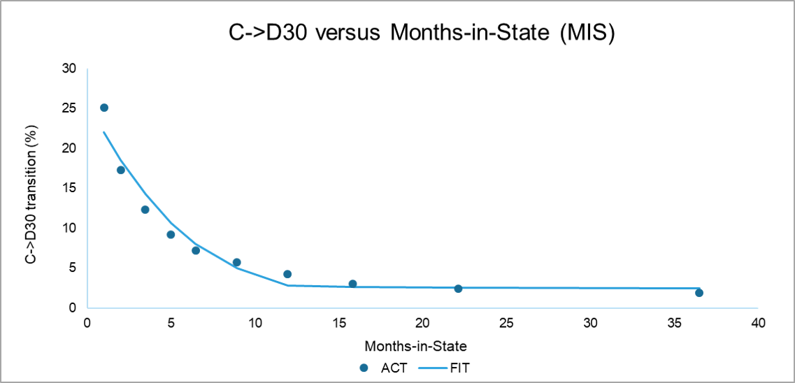
Figure 3: Impact of MIS on Blemished-C->D30 Transition (Agency Fixed Rate) Source: MIAC Analytics™
Feature 4: A Granular Foreclosure/Liquidation Timeline Model
We have also updated our treatment of foreclosure (or liquidation) timelines within the CORE Residential Model framework. Although the time from initial delinquency to final resolution of the asset is generally referred to as foreclosure timelines by practitioners, we prefer to use the term liquidation timeline. This is because our modeling approach consistently handles both the typical “foreclosure-start to foreclosure-sale to REO-liquidation” as well as more cooperative default resolutions such as short sales, deed-in-lieu, and third-party takeouts. In fact, we find that a substantial fraction of short sale default resolutions occur without ever initiating foreclosure.
Liquidation timelines are important for both whole loans (because they impact loss severities and the timing of cash flows) as well as MSR assets (because they impact sub-servicing costs, advancing expense, and reimbursement shortfalls).
Our liquidation timeline model has two distinctive features. First, it incorporates the impact of state-level geography. It is well known that liquidation timelines in Judicial states (e.g., NY) are much longer than in Power-of-Sale states (e.g., TX). However, it is perhaps less well appreciated that there is substantial variation within each of these two categories. In fact, there is substantial overlap: the fastest Judicial states have slower timelines than the slowest Power-of-Sale states. Second, although geography plays a critical role in liquidation timelines, borrower and loan attributes also play an important role. This is because overall liquidation timelines are a probability-weighted average of various liquidation outcomes. For example, NY loans with a high probability of a short-sale resolution will have shorter average timelines than NY loans with a low short-sale probability.
Additional details regarding our approach to liquidation timelines are contained in the November 2019 issue of MIAC Research Insights.
Feature 5: A state-of-the-art Loss Severity Model
Our CORE Residential Model includes an enhanced Loss Severity Model, which reflects three key improvements.
First, the loss severity model is fully integrated with the default frequency and FCL timing models. That is, the transition frequency model produces an estimate of the expected months-past-due (hereafter, MPD) conditional upon liquidation for every projection month. This expected MPD estimate is then input into the loss severity model. This seamless integration means that any attribute (or user scalar) that impacts liquidation timelines (e.g., the geographical location of the property) will automatically impact loss severity. In other words, the function of the severity model is to predict losses given liquidation timelines, while the role of the frequency model is to predict the liquidation timelines. This is precisely analogous to the way a prepayment model works. Namely, it predicts prepayments conditional upon a given realization of primary mortgage rates. Primary mortgage rate projections (either static or OAS-based) are external to the prepayment model itself.
As a recent example of the interplay between timelines and loss severities, consider the Federal CARES Act promulgated in response to COVID-19 enacted in March 2020. Under the provisions of this act, federally backed mortgage loan servicers (including those servicing conventional Agency loans) were prohibited from initiating any foreclosures for a 60-day period starting March 18, 2020. The cash flow and impact of this act were quantified within our model framework by reducing (to zero) the probability of migrating from Seriously Delinquent to REO for two observation months. As expected, this increased expected MPD and hence loss severities.
The second enhancement of our new severity model is that it is developed and estimated at the component-level. That is, we have separate estimations for the property loss and three major expense components: Taxes and Insurance, Maintenance, and Legal. This component-based approach has several advantages. First, component-level estimation is much more straightforward. Second, component-level outcomes give users more flexibility to perform “what-if” prospective analyses. For example, if prospective property taxes increase in a jurisdiction, model users can easily adjust the appropriate coefficients and quantify the impact on their portfolio. A final advantage is that it is easier to extend the model – estimated on Agency loss data – to other Sectors. For example, losses on FHA loans can be analyzed by applying a reimbursement shortfall to the legal component of total losses.
The third and final enhancement regarding the updated loss severity is the introduction of additional explanatory variables. For example, we find that loan purpose is an important driver of loss severity: purchase loans are less likely to have appraisal bias. As a result, they have lower severities than refinances, holding all other factors constant. It is plausible that the appraisal reforms included in Dodd-Frank will reduce “appraisal shopping” and hence the magnitude of this effect. However, we plan on waiting for more evidence to accumulate before we modify this effect in our model. Also, we include variables that enhance predictive accuracy even though the causal mechanism is indirect. As an example, we find that higher FICO scores result in lower loss severities, primarily through the property loss component. We attribute this to higher FICO borrowers taking better care of their properties as well as a higher percentage of cooperative resolutions, such as borrower-titled short sales.
Feature 6: Sub-Models that Capture Distinct Intra-Sector and Product-Specific Behavior
The final distinguishing characteristic of the CORE Residential Model is that we distinguish default and prepayment behavior both across and within sectors. For example, within the GNMA sector, we find that FHA loans have worse credit than VA, even after adjusting for observable attributes like DTI, FICO, and CLTV-MTM. And VA prepayments are much more sensitive to rate incentive versus FHA prepayments, especially between 6-10 months WALA. Within non-Agency, we find that non-QM loans require their own sub-sector model. In other words, even after adjusting for the large set of observable characteristics displayed in Figure 1, non-QM loans have worse credit, faster base case speeds, and lower refinance sensitivity.
Even within a sector or sub-sector, we have product-level differentiation where necessary. As an example, we find that non-Agency Hybrids have higher C->D30 transition rates than non-Agency Fixed Rates, even before reset and after adjusting for observable attributes. This is especially true of the short-reset Hybrids that were ubiquitous before the financial crisis.
Conclusions
The release of the CORE family of residential behavioral models represents an important milestone for the industry, for MIAC, and most importantly for our clients. These models are important drivers for both whole loans and MSRs, and all applications: valuation, risk sensitivities, stress testing, CECL, and beyond. Borrower behavior projected from CORE models are highly intuitive and robust in both base case and stress scenarios.
These models have been integrated with granular cash flow engines and are facilitated by the most robust data handling tools available in the industry. They provide users with the ability to precisely quantify the implications of specific loan attributes and macroeconomic scenarios across a diverse set of Residential assets.
These enhanced models will enrich valuations and risk metrics for software, valuation and hedge advisory clients.
MIAC Perspectives: Introducing the Updated CORE™ Residential Models for Credit, Prepayment, and Loss
Author
Dick Kazarian, Managing Director, Borrower Analytics Group
Dick.Kazarian@miacanalytics.com