By Dick Kazarian, Managing Director, Borrower Analytics Group
Introduction and summary
In our Winter 2021 edition of MIAC Perspectives, we provided an overview of our updated CORE™ Residential Models for Credit, Prepayment, and Loss. We identified six major features which distinguish these CORE models from alternative models available in the analytics marketplace. In the latest edition of MIAC Perspectives, we take a closer look at one of these important distinctions: our methodology for handling Liquidation timelines. We cover the following topics:
- The mechanics of liquidation timelines in our CORE framework
- Why foreclosure timelines don’t tell the whole story
- What factors drive liquidation timelines
- How have timelines been impacted by COVID
- How do timelines impact whole loans
The mechanics of liquidation timelines in our CORE framework
We define the liquidation timeline for a residential loan to be the number of months it takes to resolve a distressed asset, from initial delinquency through final resolution. An important complication is that a loan can liquidate with a loss via many possible paths – and each of these paths has different potential timelines.
To explain the relationship between a transition model and liquidation timelines, a little background is needed. The role of a transition model is to project the future evolution of a loan based on the loan attributes and the macro-economic assumptions. In other words, the model needs to predict the probabilities of all feasible delinquency statuses every month in the future. For example, consider a loan that starts out as current (i.e., C). The transition model will predict the probability that the loan remains current, misses a payment, and transitions to D30, or prepays at the end of the month.
In any transition model, liquidation and prepayment are inactive (or terminal) statuses. In other words, once a loan transitions to either a loss liquidation or a prepayment, it remains inactive. In contrast, serious delinquency (SDQ) and REO are active statuses. For example, consider a loan that is currently four months delinquent (i.e., D120). That loan can cure to a less delinquent state, remain in D120 by making a payment, miss a payment and thus migrate to D150, or liquidate with a loss.
Figure 1 shows the transition possibilities that exist in our CORE transition model framework. Following standard practice, the rows display the loan status at the beginning of the month (i.e., BOM) while the columns display the end of month status (i.e., EOM). For example, starting from Current (i.e., C), a loan can transition over the next month to three possible future statuses: D30, PIF (i.e., paid-in-full), or C (i.e., remain current). Figure 1 also displays the distinction between active states and the inactive states of PIF and LIQ (loss liquidation).
As Figure 1 makes clear, there are two ways that a loan can incur a loss liquidation. This first is to migrate to REO and then proceed to a liquidation of that REO. In this case, the servicer takes title to the collateral and then proceeds to sell it. Empirically, these resolutions are overwhelmingly completed foreclosures, but also include a small number of deed-in-lieu resolutions. A second possibility is an immediate transition from D120+ to liquidation. In this case, the servicer never takes title to the REO. These resolutions are mostly borrower-titled short sales, but also include a small number of third-party take-outs and write-offs.
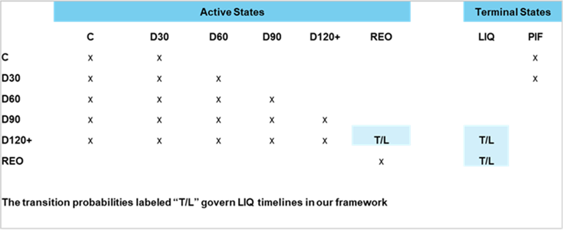
Figure 1: CORE Transition Model Framework
Liquidation timelines are an output – not an input – of our framework
Within our transition framework, there is a one-to-one correspondence between these transition probabilities and average liquidation timelines. The lower the probability of leaving serious delinquency (here, defined as D120+), the longer it will take, on average, to liquidate. And the longer it takes to liquidate, the higher will be the expected months delinquent when liquidation does finally occur. We designate the primary transition probabilities governing these timelines with a “T/L”.
Stated differently, liquidation timelines are an outcome of our model, not an input to the model. This is the only way to maintain consistency within a transition model framework.
To see this, consider a simplified framework where loans can only liquidate from a completed foreclosure and subsequent REO liquidation. In that case, the average liquidation timeline will be driven entirely by two transition rates: D120->REO and REO->LIQ. Any loan attribute or macro-economic factor which reduces those transition rates will increase the average amount of time the loan spends in D120+ or REO, and thus increase average liquidation timelines. In the more complex structure underlying our CORE Residential Valuation Model, average liquidation timelines will also depend on the resolution mix predicted by the model.
Why foreclosure timelines don’t tell the whole story
Since liquidation can occur either through REO (i.e., Foreclosure) or non-REO (i.e., short sales), average timelines will be a mixture of these two resolution types. And short sale timelines are considerably shorter than REO timelines, especially in Judicial states. This distinction would not be important if short sales were rare. However, short sales are a large and growing component of overall liquidations. The relative importance of short sales is displayed in Figures 2-4. We extracted monthly transition rates on D120+ loans from the FHLMC single-family LLD dataset with observation dates between January 1999 and December 2019. These data were selected to exclude the COVID period. Figure 2 plots the D120->REO transition rate, while Figure 3 plots the D120->LIQ transition rate. The most obvious takeaway is that D120->REO rates have declined continuously since hitting a peak before the Great Financial Crisis (i.e., GFC). In sharp contrast, D120->LIQ rates have increased dramatically since 2012 (in part because of the Servicer Settlement). Figure 4 displays the ratio of these two outcomes. As is evident, the short sale to REO resolution ratio has increased ten-fold from 0.25 to 2.5! We limited the sample to Judicial states, but the overall patterns for the power of sale (i.e., POS) states are very similar, except that the D120->REO rates for POS states are generally higher.
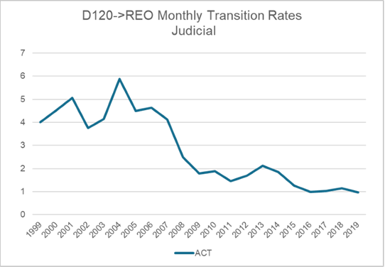
Figure 2: D120->REO Monthly Transition Rates (Judicial States)
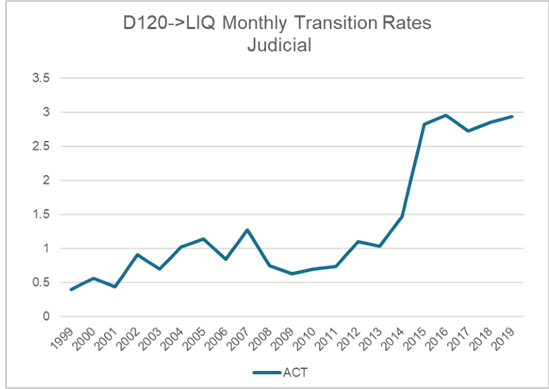
Figure 3: D120->LIQ Monthly Transition Rates (Judicial States)
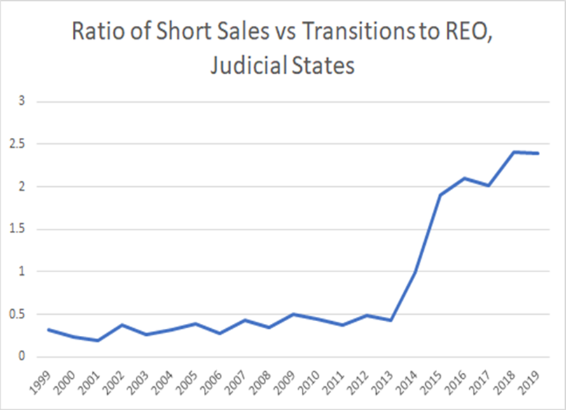
Figure 4: Ratio of Short Sales vs Transitions to REO (Judicial States)
The overall conclusion from the above discussion is that ignoring the resolution mix and focusing exclusively on foreclosure timelines alone will result in Liquidation timeline estimates that are too long. And with collateral with a high propensity for short sales in slow Judicial states, this over-estimate can be quite large. Moreover, there is good reason to believe that with continuing foreclosure moratoria and new CFPB servicing guidelines, short sales may play an even bigger role in the future.
Our CORE model projections reflect the importance of short sales
Another way to see the relative importance of short sales is to analyze projections from our CORE model. We selected a hypothetical moderately seasoned FHA loan (age = 35 months), with a $350k balance, FICO=575, DTI=45, and an MTM LTV of 110. The initial delinquency status was assumed to be clean current. These weak credit attributes imply a cumulative liquidation rate of about 12%. We then ran this loan in an average Judicial state and an average POS state. The liquidation results are displayed in Figure 5. At each liquidation month, we show the REO and short sale (i.e. SS) mix conditional upon liquidation. Several conclusions are apparent. First, there is no possibility of a short sale liquidation until month 5, and no possibility of an REO liquidation until month 6. Second, short sale liquidations dominate early on, and especially so in Judicial states. Third, even after 24 months, short sales continue to comprise a significant fraction of total liquidations.
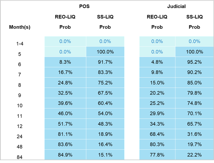
Figure 5: Probability of Liquidation Type by liquidation Month
One implication of this changing mixture is that average Liquidation timelines will increase over time. Although these are probabilities projected by our model, one can think of these as the average outcomes from a homogeneous pool of loans with the above characteristics. In a geographically diverse pool, the changing resolution mixture would be much more dramatic.
What factors drive liquidation timelines
Any factor that impacts the three key transitions (D120->REO, D120->LIQ, and REO->LIQ) will impact the average Liquidation timeline. These factors include loan attributes (e.g., high FICO loans are more likely to short sale), the property’s geographical location, and even the economic environment (e.g., lower home prices and higher unemployment extending timelines). In a subsequent Issue of MIAC Perspectives, we’ll delve into these topics in greater detail. For now, we’ll just highlight a few important takeaways.
Figure 6 shows the importance of time spent in serious delinquency (which, as noted above, we define to be D120+). Generally speaking, the longer the loan has spent in D120+, the less likely it is to migrate to REO. This is true for both Judicial and POS states, but the pattern is somewhat different. The “humped” pattern for Judicial states motivated our decision to develop separate models for the two groups. Note also that our D120->REO model fits the data quite well. Finally, while time-in-state is input data for D120+ loans as of the launch date of the projection, this variable needs to be propagated consistently within the forward simulation. Although this involves additional run-time computations, the increased accuracy justifies the effort.
Figure 7 shows that there is considerable variability within the broad Judicial/POS dichotomy. We divide monthly D120->REO transitions into more granular state sub-groupings and list some of the larger states within each sub-group. For example, the slowest POS states (e.g., CA and MA) have average D120->REO rates of only 1.9 – which is similar to the typical Judicial state. The fastest POS states are nearly three times faster (at 5.5%). We see the same dispersion among Judicial states, with NY and NJ being the slowest by far. Note the significant amount of dispersion across state sub-groups: the fastest POS states are 10 times faster than the slowest Judicial states (5.5 v. 0.5).
In addition, our research shows that there is substantial variability in D120->REO transitions within states. For example, NYC is substantially slower than NY as a whole. Similarly, Miami Dade county is much slower than FL overall. These geographically based observations are particularly important because many portfolios which MIAC analyzes – either in our whole loan or MSR valuation groups – are geographically concentrated. And the implications for NPLs or low credit quality RPLs can hardly be overstated.
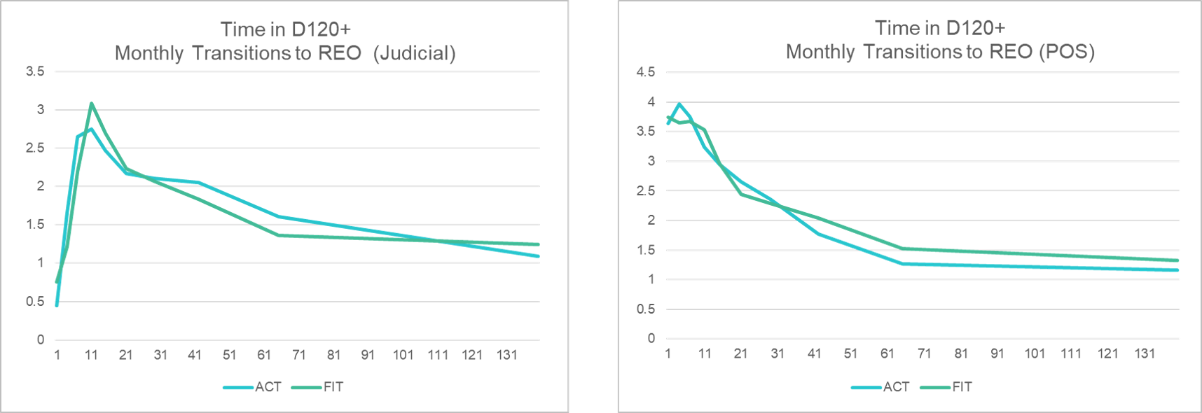
Figure 6: Time in D120+ Monthly Transitions to REO (Judicial) and Time in D120+ Monthly Transitions to REO (POS)
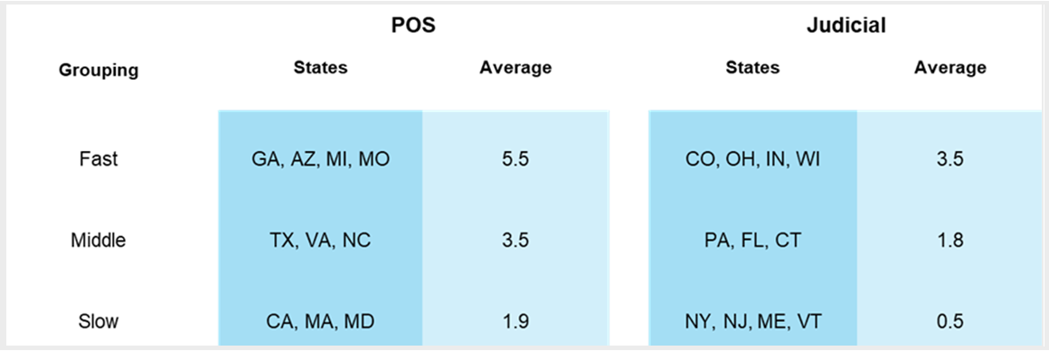
Figure 7: Variability within the POS and Judicial Segments
How have timelines been impacted by COVID
It is well known that policy risk is a major consideration in mortgage analysis, and COVID has provided yet another example of this exposure. As a result of forbearance mandates, foreclosure and eviction moratoria, servicing guideline updates, and other factors, migrations from D120+ to either REO or LIQ had collapsed by March 2020 and have not yet recovered to pre-pandemic levels. Figure 8 shows the conventional D120->REO transition rates for Judicial states, and Figure 9 shows the D120->LIQ rates during the COVID period. POS states exhibit the same pattern; details are omitted.
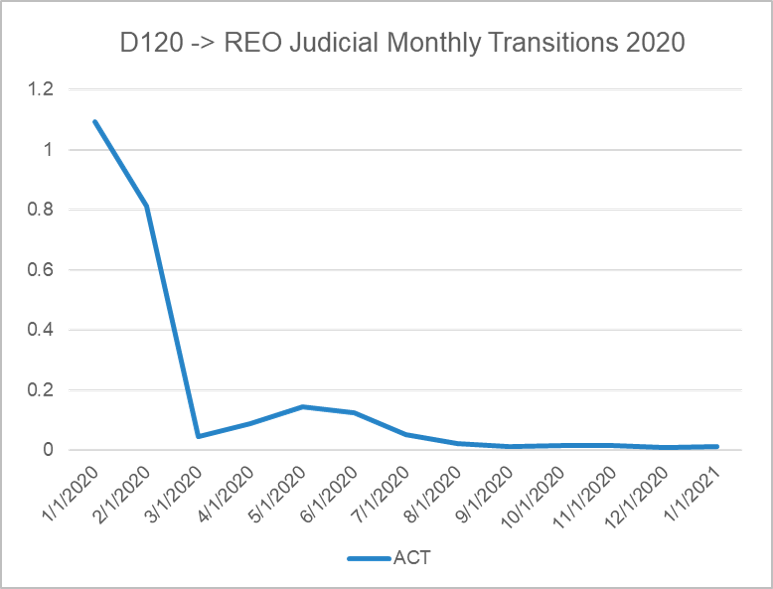
Figure 8: D120->REO Judicial Monthly Transitions 2020
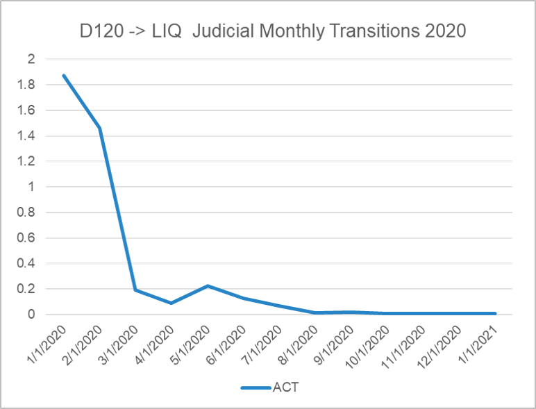
Figure 9: D120 ->LIQ Judicial Monthly Transitions 2020
Impact on whole loans
Whole loan investors should be concerned about Liquidation timelines because longer timelines imply (1) a longer period to recover funds on a defaulted loan and (2) a lower net recovery rate when the funds are ultimately received (i.e., a higher loss severity). And the higher the probability of default, the greater the impact will be. In the extreme case of an NPL where default liquidation is almost certain, lower recoveries will lower prices on a roughly dollar-for-dollar basis.
As we indicated in the Winter 2021 Issue of MIAC Perspectives, our CORE loss severity model has numerous advantages over many competing analytical frameworks. These strengths include a great fit to the historical loan-level loss data, component-level projections, full integration with our transition model, and a full array of explanatory variables. In this section, we’ll just highlight the marginal impact of timelines on losses.
To display the impact of Liquidation timelines on Loss Severity, we took a hypothetical conventional loan with the following characteristics: UPB=300k, LTV=90, Loan Purpose = Purchase, and a note rate of 3.75%. We then varied the inputted Liquidation timeline into our CORE severity model, holding all other factors fixed, and computed the marginal effect of timelines on each loss severity component.
The impact of Liquidation timelines is displayed in Figure 10. Timelines (represented as months past due, or MPD) is contained in the first column. The first panel shows the impact of MPD on the loan, assuming the property is domiciled in NY state. We display four components of loss severity: property loss, taxes and insurance (T+I), Maintenance, and Legal fees. Delinquent accrued interest is directly proportional to MPD, does not require any estimation, and is not displayed here. The second panel examines the same loan, but the computations assume the property is located in CO.
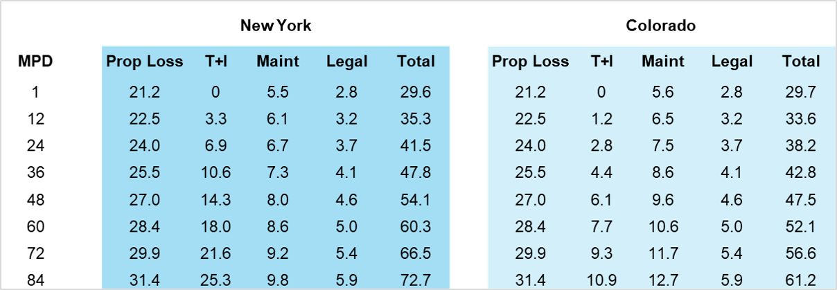
Figure 10: Liquidation Timelines: Impact on Whole Loan Loss Severities for NY and CO
Several points regarding Figure 10 merit consideration. First, property losses actually increase with MPD, likely due to accumulated deferred maintenance or even active malevolence on the part of homeowners or non-owner occupants. Second, the tax and insurance components are directly proportional to MPD. Further, the slope is higher in higher tax jurisdictions (like NY). Relative to CO, this means that NY has two distinct disadvantages: it has longer average timelines and it has higher T+I costs per MPD.
Third, similar to T+I, maintenance expenses increase proportionately with timelines. In contrast to T+I, Maintenance expenses are significant even with immediate liquidation (i.e., MPD=1). Note also that CO has somewhat higher Maintenance expenses per MPD than NY, but this is more than offset by NY’s significantly higher T+I. Furthermore, the effects of T+I and Maintenance are LTV-dependent. Although low LTV loans are less likely to incur a default liquidation, they will incur higher T+I and Maintenance costs relative to UPB if liquidation occurs. Finally, legal expenses increase with MPD. But like Maintenance expenses, legal expenses can be substantial even if timelines are very short.
There is much more to say about Liquidation timelines, their impact on both whole loans and MSRs, and our loss model. We’ll save these topics for future editions of MIAC Perspectives.
MIAC Perspectives: A Closer Look at Liquidation Timelines in MIAC’s CORE™ Models
Author
Dick Kazarian, Managing Director, Borrower Analytics Group
Dick.Kazarian@miacanalytics.com