By Dick Kazarian, Managing Director, Borrower Analytics Group
This article takes a closer look at some key features of our updated Agency Credit Model within our CORE™ Model Suite. Also highlighted are unique behaviors that occurred during the COVID period.
Framework
Figure 1 shows the transition model framework used by the latest version of our CORE model. We track each loan’s contractual delinquency status from current (C) through serious delinquency (D120+). This granular description of a loan’s delinquency status is critical for accurate valuation of seasoned whole loans (especially re-performing and non-performing loans), as well for MSRs.
As a reminder to readers, we use the notation “A->B” to denote a transition from status A to status B. For example, C->D30 refers to a migration from current to D30. Similarly, D60->C denotes a cure from D60 to current (i.e., the borrower made three payments over the month).
The delinquency status as of the valuation launch date is a vital driver of subsequent performance. For example, a loan that is D90 (i.e., 3 months past due) is far more likely to eventually default than a loan that is D30 as of the analysis date. Additionally, the time-in-status (i.e., months-in-state) is also important, as D30 loans which have persisted in D30 for many months (rolling D30s) are much more likely to remain in D30 than to either cure or migrate to D60.
It is worth noting that this framework allows us to consistently analyze any loan, including REO assets, with any delinquency status. We’ll delve into that topic, together with some model sensitivity analysis, in a subsequent article.
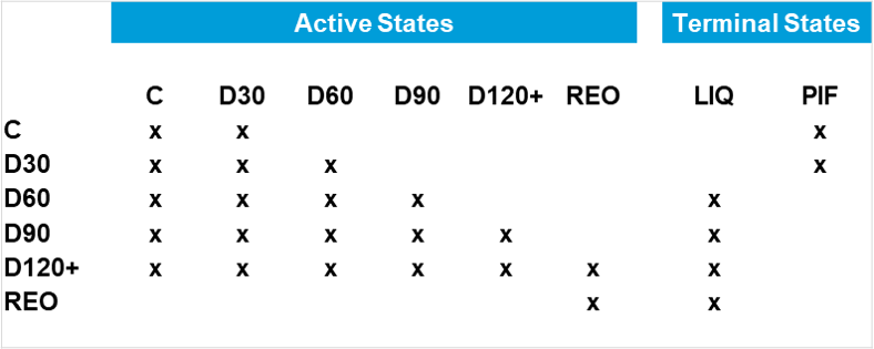
Figure 1: CORE™ Model Framework Source: MIAC Analytics™
Why is the Agency Credit Model so important?
The Agency Credit Model forms the backbone of our CORE Model Suite because the underlying datasets are the most comprehensive. An ideal development dataset for residential mortgages has the following four key characteristics: 1) variation in attributes, 2) detailed static attributes, 3) ability to track loan performance from origination though final disposition, and 4) origination and observation dates covering multiple economic scenarios.
Variation in Attributes
The Agency data has wide variation in DTI, FICO, LTV, Balance, and other attributes. Both intuition and formal statistical analysis indicate that, unless there is variation in DTI, it will be impossible to infer the impact of DTI on mortgage outcomes.
Detailed Static Attributes
The Agency data has a comprehensive set of origination attributes, including a co-borrower flag, which is an important driver of credit transitions.
Ability to track loan performance from origination though final disposition
We can track Agency loans through their final resolution in the event of a default. In contrast, the loan-level GNMA pool-factor data does not track loan performance once the loan exits the pool. This makes liquidation time estimation virtually impossible within the GNMA sector. As we’ve indicated previously, liquidation timelines are a significant driver of loss severities for whole loans and for sub-servicing costs for MSRs.
Origination and observation dates covering multiple economic scenarios
The Agency data extends back to the late 1990s, well before the GFC and the associated HPA decline. This means we can estimate the behavior of loans with mark-to-market LTVs (i.e., CLTV-MTM) exceeding 150 or more. In contrast, the loan-level GNMA and post-crisis non-Agency data have only seen home price increases.
The transition probabilities are estimated using two overlapping sources of loan-level Agency data: 1) the pool factor data (from eMBS), and 2) the Single-Family Loan-Level dataset distributed directly by the GSEs themselves. The quality and extent of the combined Agency data enable us to estimate very detailed relationships that are not possible with the GNMA and Non-Agency data. Our general approach is to use these Agency estimates to inform those relationships in other sectors. In fact, this approach is used by virtually all mortgage analysts.
Each probability transition displayed in Figure 1 is estimated separately. This allows the historical data to tell the story, rather than to impose potentially erroneous assumptions on the model specification. In our Winter 2022 Issue of MIAC Perspectives, we indicated how important that flexibility was in the context of disentangling the impact of Occupancy on cumulative default liquidations.
What Drives C->D30?
Although ultimate loan outcomes are driven by all the transitions displayed in Figure 1, the C->D30 model is by far the most important transition for loans that are contractually current as of the analysis launch date.
Before turning to the results of our estimation, it is important to observe that we need to create fully separate (i.e., segmented) models for loans that are always current (AC) vs loans that are dirty current (DC). By dirty current, we mean loans that are re-performing (i.e., that have had one or more prior delinquency episodes, but have subsequently self-cured). Loans that cure through a modification are handled in a separate framework.
How did we arrive at this need for segmentation? In this specific case of C->D30, it turns out that this phenomenon has been well-established among experienced mortgage researchers for more than a decade. To our knowledge, the first published work dates back to a Barclays Capital paper authored by Steven Bergantino and published shortly after the GFC. But in general, the need for segmentation has been established by our model development process, which is described in our CORE Model Documentation. There are many other examples of the need for model segmentation, most notably in the liquidation timeline models.
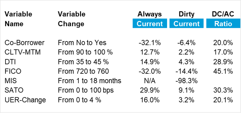
Figure 2: Impact of selected attributes on C->D30 transition (%) Source(s): eMBS, FHLMC LLD, MIAC Analytics™, MIAC Internal calculations
Some selected empirical results are summarized in Figure 2 for the AC->D30 and DC->D30 transitions. The table is structured as follows. The “Variable” column displays key explanatory factors along the rows, and the “Variable Change” column defines a hypothetical change in that variable. Finally, we show the percentage impact on the AC->D30 and DC->D30 transitions for that given hypothetical change in the explanatory variable. These percentage impacts depend upon the base case levels, which we define as the sample average.
Several conclusions are apparent from this table. First, the percentage impact of each variable on outcomes are much smaller for the DC->D30 transition than for the AC->D30 transition. Once a loan has had a prior delinquency episode, these other attributes convey much less information. Second, all the impacts have the same sign for both models. Third, the relative information decay varies substantially across attributes. This is displayed in the final column, which shows the ratio of the impact on the DC and AC models. Note that the lowest information loss is still high (55% for FICO), and the greatest information loss occurs with CLTV-MTM. The latter is due, in part, to the heterogeneity of individual home prices around the HPA Index.
Finally, observe the enormous importance of the months-in-state (MIS) variable on DC->D30. Loans that have been re-performing for 18 months are far less likely to migrate to D30 again, relative to loans that have been re-performing for 2-3 months. However, re-performers are always worse than never delinquent loans. We omitted statistical standard errors in the table, but all coefficients are significant at the 1% level.
A Closer Look at Unemployment and C->D30 Transitions
From Figure 2, it is also evident that unemployment change (UER-Change) has a significant impact on
AC->D30 transitions. We measure UER-Change as the difference between the UER level as of the observation date, less the UER level as of loan origination. Our empirical research shows that this is a much better specification than the UER level itself, and this is also consistent with economic intuition. This is yet another example of the importance of defining explanatory factors (or features) carefully in any empirical investigation.
Figure 3 shows that, if we exclude the COVID period (which, for simplicity, we consider 2020-2021), the model fits the data very well. That is, the actual AC->D30 transitions track the fitted AC->D30 transitions very closely. However, this relationship breaks down over the 2020-2021 COVID period, as exhibited in Figure 4. Figure 5 repeats the analysis displayed in Figure 3 for Dirty Current loans excluding the COVID period. Again, we see a clear relationship between DC->D30 and UER-Change as well as the solid performance of our estimated model. We can also see that average DC->D30 rates are much higher than average AC->D30 rates, as well as the lower UER sensitivity. Figure 6 repeats the analysis exhibited in Figure 5 for the COVID period. Once again, the relationship breaks down over that two-year period, just as we saw with the AC->D30 transitions.
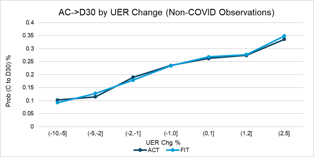
Figure 3: AC->D30 transition by UER-Change, Actual v. Fitted, Non-COVID Period Source(s): eMBS, FHLMC LLD, MIAC Analytics™, MIAC Internal calculations
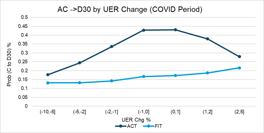
Figure 4: AC->D30 transition by UER-Change, Actual v. Fitted, COVID Period Source(s): eMBS, FHLMC LLD, MIAC Analytics™, MIAC Internal calculations
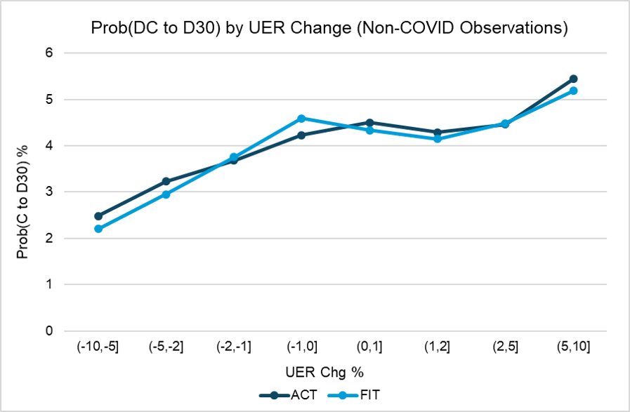
Figure 5: DC->D30 transition by UER-Change, Actual v. Fitted, Non-COVID Period Source(s): eMBS, FHLMC LLD, MIAC Analytics™, MIAC Internal calculations
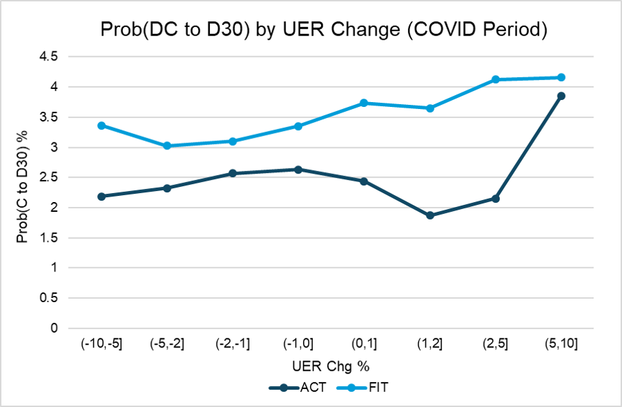
Figure 6: DC->D30 transition by UER-Change, Actual v. Fitted, COVID Period Source(s): eMBS, FHLMC LLD, MIAC Analytics™, MIAC Internal calculations
Figures 7-8 show the same phenomena from a time series perspective (that is, across observation dates). As is evident, there was a sudden sharp spike in both AC->D30 and DC->D30 transition rates in early 2020 as the pandemic unfolded.
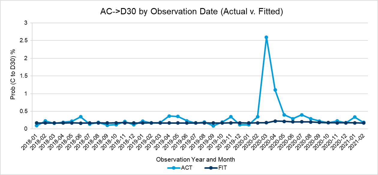
Figure 7: AC->D30 transition by Observation Date, Actual v. Fitted Source(s): eMBS, FHLMC LLD, MIAC Analytics™, MIAC Internal calculations
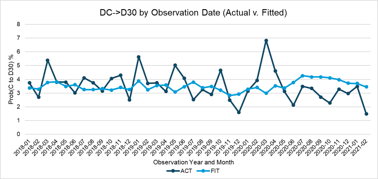
Figure 8: DC->D30 transition by Observation Date, Actual v. Fitted Source(s): eMBS, FHLMC LLD, MIAC Analytics™, MIAC Internal calculations
What explains this aberrant COVID behavior?
The sharp increase in C->D30 rates was primarily the result of the widespread availability of Borrower Assistance (i.e., Forbearance) Plans. These were widely advertised through a variety of channels as the pandemic unfolded. These plans completely removed the usual costs and consequences of becoming delinquent. First, late fees could not be assessed. Second, servicers reported contractually delinquent mortgages as current to the credit repositories, so credit reports and FICO scores were not impacted. In fact, we were surprised that the uptake on these plans was not more widespread. Another reason for the increase in C->D30 rates is that some borrowers experienced income disruptions during COVID, at least temporarily.
What about the breakdown of the relationship between UER-Change and C->D30? In general, increases in UER result in higher C->D30 rates. This occurs because borrowers who become unemployed see income decreases. But that is not what happened during COVID. UER gapped higher, but the US Government dispensed generous COVID-related stimulus payments. The Federal Pandemic Unemployment Compensation supplement contained in the CARES Act is one prominent example. An interesting analysis by the Becker Friedman Institute (Working Paper 2020-62) estimated that a large fraction of unemployed persons experienced increases in income as a result of their job loss. As a result of these income replacement rates exceeding 100%, the usual relationships broke down, as displayed in the above Figures.
What steps are needed to ensure accurate model projections?
First, we must ensure that our estimates are correct. Whenever a non-recurring event occurs in the historical data, there is the potential for contamination of statistical estimates that seek to describe the normal expected relationships. The safest and most consistent approach is to drop those observations from the estimation dataset. This is the approach we adopted in the update of our Agency Credit Model.
Second, we must ensure that the run-time invocation of our model is not compromised by the aberration itself. To see what’s at stake, consider a loan originated in 2020-05 when the official national UER rate was 13%. Later, in 2022-04, UER had dropped to 3.3%. We would not want to calculate a UER-Change of -9.7 and feed it into our CORE model, as that would give implausibly low forecasts for future C->D30 rates. We have made the appropriate adjustments to our handling of COVID-era loans to avoid these and related issues.
Conclusion
This article takes a closer look at our new Agency Credit Model. Although there are many issues that merit consideration, we decided to focus on the few that were both important and timely. They include:
- Flexible Model Framework that enables consistent evaluation of all residential assets at any stage of delinquency, including REO
- Importance of an Agency Credit Model within the suite of CORE models
- Advantages of the Agency development dataset and the limitations of other sector datasets
- Importance of model segmentation generally, and specifically with respect to Always Current vs Dirty Current
- Impact of Unemployment on credit transitions, even after adjusting for home prices
- Aberrant behavior of C->D30 rates during the 2020-2021 COVID period
- Remediation steps for handling the COVID period, which include run-time model usage
MIAC Perspectives: CORE Insights: A Deep Dive into our Agency Credit Model and the Impact of COVID-19
Author
Dick Kazarian, Managing Director, Borrower Analytics Group
Dick.Kazarian@miacanalytics.com
View MIAC Perspectives – Spring 2022 Issue