By Dick Kazarian, Managing Director, Borrower Analytics Group
As noted in our Market Overview, the FHFA has announced significant changes to the LLPAs for Second Homes effective April 1, 2022. In this article, we take a closer look at the impact of Occupancy type within our CORE™ Agency model, with a focus on Second Homes.
Framework
Figure 1 shows the transition model framework used by the latest version of our CORE model. We track each loan’s contractual delinquency status from current (i.e., C) through serious delinquency (i.e., D120+). This granular description of a loan’s delinquency status is critical for accurate valuation of seasoned whole loans (especially re-performing and non-performing loans), as well as valuation of MSRs. The transition probabilities are estimated using two overlapping sources of loan-level Agency data: the pool factor data (from eMBS) and the Single-Family Loan-Level Dataset distributed directly by the GSEs.

Figure 1: CORE Model Framework Source: MIAC Analytics™
Delinquency Transitions
Each probability transition displayed in Figure 1 is estimated separately. This allows us to let the historical data tell the story, rather than to impose potentially erroneous restrictions. As we demonstrate below, this flexibility turns out to be critically important in the case of Occupancy type.
We find that Second Homes and Investor Properties have lower C->D30 transition rates than Primary Homes, holding all other attributes constant. Second Home C->D30 transition rates are approximately 15% lower, and Investor Properties are approximately 16.5% lower. Similarly, non-Owner-Occupied loans (hereafter, NOO) have higher self-cure rates (i.e., D30->C) by 12-14%. These results are intuitive, as these borrowers have better unobserved attributes, such as higher levels of non-housing wealth and a generally higher level of financial sophistication.
However, once a loan hits D60 or worse, NOO loans have worse credit transitions. Specifically, they are more likely to miss their next payment (e.g., they have a higher probability of D60->D90), and less likely to cure (e.g., D60->C). For example, Second Homes have a 14% higher D60->D90 transition, and Investor Properties have a 31% higher D60->D90 probability. What explains this reversal in the impact of Occupancy type? We believe the reason is unobserved trigger events. If a Second Home hits D60 or worse, there is a decent chance that some adverse event has occurred (e.g., divorce or job interruption).
So, while a Second Home is less likely to ever hit D60 starting from current, it will perform worse if it does. In contrast, Primary Occupancy borrowers are much more likely to use their mortgage delinquency to manage cash flows. This means that a D30 or D60 is less likely to signal an underlying trigger event. As an obvious example, a borrower can skip payments for 2-3 months as a type of short-term borrowing. Although the costs are significant (including late fees and negative impact on credit score), there is no risk of losing one’s home.
Another difference across Occupancy types is that NOO loans have much shorter average liquidation timelines, for two reasons. First, they are more likely to resolve via a short sale rather than a completed foreclosure and REO liquidation. Second, conditional on going through REO, they progress much faster. This is yet another example of a point we’ve made repeatedly: expected liquidation timelines depend upon borrower, loan and property characteristics, in addition to the geographical location of the property.
A summary of key impacts for NOO is displayed in Figure 2.
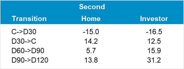
Figure 2: Impact of NOO on Selected Transitions in Agency CORE (%) Source: MIAC Analytics™
Cumulative Liquidations
As noted above, NOO loans have better early-stage credit transitions and worse late-stage credit transitions. In order to determine the net effect on cumulative liquidations (hereafter, CUM-LIQ), we ran a set of benchmark loans through our CORE Agency model. Cumulative liquidation is the probability that a loan liquidates with a loss at any time in the future. In all cases, we compared new originations as of the analysis launch date with typical Agency characteristics. A comparison of Second Homes and Primary Occupancy for various LTVs is displayed in Figure 3. We varied LTV-MTM by fixing the UPB and changing the home price. In order to display the full range of model behavior, we examined extreme values of LTV-MTM that would not, of course, be observed at origination.
As expected, CUM-LIQ increases as LTV-MTM increases for both Occupancy types. However, Second Home CUM-LIQ are always lower than Primary Home CUM-LIQ, with the ratio in the 86-90% range. We get similar results from other perturbations, such as FICO or UPB. These results demonstrate that, for new originations, the better credit migrations at earlier delinquencies dominate the worse credit migrations at D60 and below. Of course, for seasoned loans starting at D60 or worse, Second Homes would have higher CUM-LIQ than Primary.

Figure 3: Comparison of Second Home versus Primary Occupancy by LTV Source: MIAC Analytics™
Cumulative Losses
Figure 3 also displays cumulative losses (hereafter, CUM-LOSS). This is defined as the (undiscounted) expected dollar loss on the loan divided by the UPB as of the launch date. It can be interpreted as the CUM-LIQ multiplied by the average Severity (hereafter, SEV). To simplify the exposition, we display collateral severities here (i.e., prior to the application of PMI). For each Occupancy type, average SEV increases as LTV-MTM increases. However, Second Home SEVs are somewhat higher than Primary SEVs, especially at lower LTV-MTM. This is true even though Second Home timelines are generally faster than Primary timelines. The higher SEVs for Second Homes have been noted by other researchers and are primarily driven by lower levels of net proceeds from liquidation.
For most levels of LTV-MTM, the higher SEVs for Second Homes means that CUM-LOSS differences are smaller than CUM-LIQ differences. However, a closer examination of the results at LTV-MTM of 70 and below shows an interesting example of reversal. In particular, at these low LTV-MTM levels, Second Homes actually have worse CUM-LOSS than Primary Homes. This is because their SEV disadvantage offsets their CUM-LIQ advantage, albeit by a small amount.
Conclusion
The recent LLPA changes motivated us to highlight and detail the impact of Occupancy on credit performance in our CORE Agency model, with a focus on Second Homes. For new production loans, credit performance for Second Homes is generally better, with the exception of very low LTV loans (where losses are small regardless). These results reinforce our earlier statement that the LLPA changes have nothing to do with expected credit losses and everything to do with a desire for more cross subsidization.
Also, as the above insights make clear, the impact of Occupancy on credit performance is highly nuanced. Second Home NPL loans that are D60 or worse as of the valuation date have higher credit losses than Primary Homes. This highlights the need for flexibility in the specification and estimation of behavioral models within residential mortgages.
MIAC Perspectives: CORE Insights: A Closer Look at the Impact of Occupancy
Author
Dick Kazarian, Managing Director, Borrower Analytics Group
Dick.Kazarian@miacanalytics.com